A surprising number of posts on this blog secretly run on the same primitive. Hashing for linear functions estimates an inner product after scrambling coordinates. Random kitchen sinks estimate a kernel value by averaging random features. Strip the applications away and one small question is left standing: given two unit vectors \(u, v \in \mathbb{R}^n\), estimate \(\rho = u^\top v\) cheaply, via functions \(f\) and \(g\) with
\[\mathbb{E}[f(u)\,g(v)] = u^\top v.\]
The split into two separate functions is the whole point. In retrieval, one side is a database of a billion vectors, compressed once and stored. The other side is a query that shows up later. The two sides never meet until the final multiply, so each must be sketched on its own, and the only thing they share is the random seed. (Unit length is no real restriction: if your vectors are not normalized, store their norms, that is one extra float each.)
Only two dimensions matter
One line of preparation does all the work below. Write \(v = \rho u + \sqrt{1-\rho^2}\, u_\perp\), where \(u_\perp\) is a unit vector orthogonal to \(u\). Draw \(w \sim \mathcal{N}(0, I)\) and set \(a = w^\top u\) and \(c = w^\top u_\perp\). Then \(a\) and \(c\) are independent standard normals, and
\[w^\top v = \rho\, a + \sqrt{1-\rho^2}\, c.\]
Only the two-dimensional shadow of \(w\) on the plane spanned by \(u\) and \(v\) ever matters. The three estimators below are bookkeeping on top of this line.
Gauss on Gauss
The classical recipe: \(f(u) = w^\top u\) and \(g(v) = w^\top v\). Unbiasedness takes one line, \(\mathbb{E}[f(u)\, g(v)] = u^\top \mathbb{E}[w w^\top] v = u^\top v\). The variance is barely longer. By the decomposition,
\[f(u)\,g(v) = \rho\, a^2 + \sqrt{1-\rho^2}\, a c.\]
The two terms are uncorrelated since \(\mathbb{E}[a^3 c] = 0\), and with \(\mathrm{Var}[a^2] = 2\) and \(\mathrm{Var}[ac] = 1\) we get
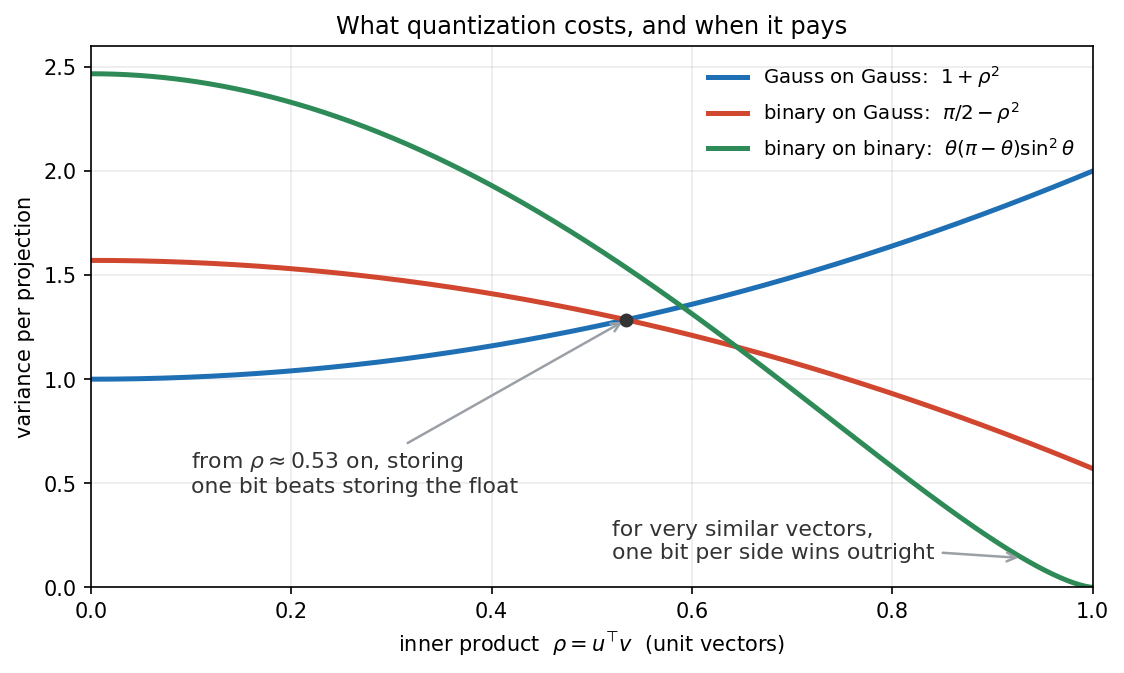
\[\mathrm{Var}[f(u)\, g(v)] = 2\rho^2 + (1 - \rho^2) = 1 + \rho^2 \leq 2.\]
Average \(\ell\) independent projections and the variance drops below \(2/\ell\), regardless of the dimension \(n\). Set \(u = v\) and the same estimator recovers squared norms. Do this for all pairwise differences among \(m\) points, add a Chernoff bound and a union bound, and you have the Johnson-Lindenstrauss lemma: \(\ell = O(\epsilon^{-2} \log m)\) dimensions preserve all pairwise distances. The same estimator powers locality sensitive hashing, where Indyk and coauthors turned random projections into sublinear-time nearest neighbor search (their CACM survey is a good entry point).
Binary on binary
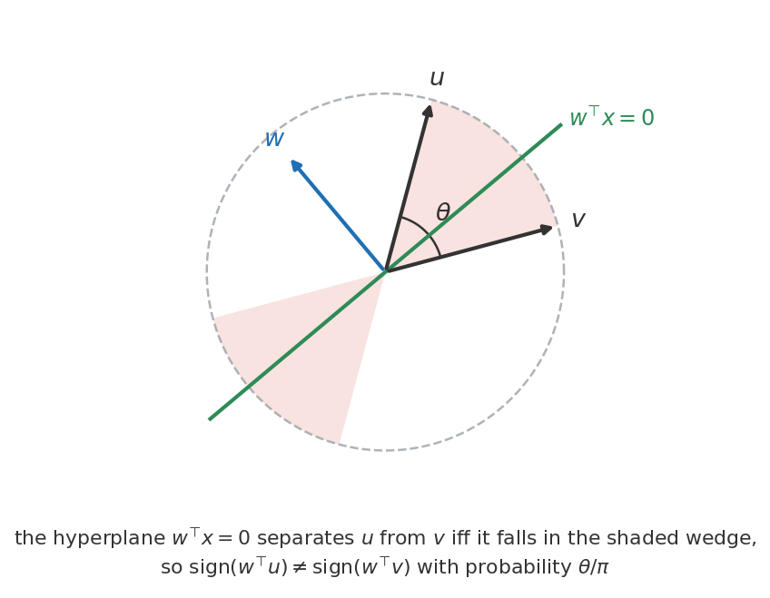
Now quantize both sides to a single bit: \(f(u) = \mathrm{sign}(w^\top u)\) and \(g(v) = \mathrm{sign}(w^\top v)\). The product is \(\pm 1\), so \(\mathbb{E}[f g] = 1 - 2 \Pr(\text{signs differ})\). The signs differ exactly when the hyperplane orthogonal to \(w\) separates \(u\) from \(v\). Only the direction of \(w\) inside the plane spanned by \(u\) and \(v\) matters, that direction is uniform on the circle, and it splits the two vectors with probability \(\theta/\pi\) for \(\theta = \arccos \rho\). Hence
\[\mathbb{E}[f(u)\, g(v)] = 1 - \frac{2\theta}{\pi} = 1 - \frac{2}{\pi} \arccos(u^\top v).\]
That is not the inner product, but it is a monotone function of it: average the bit products into \(\hat{m}\) and report \(\hat{\rho} = \cos\big(\tfrac{\pi}{2}(1 - \hat{m})\big)\). If you skip the inversion and use the raw sign agreement as a similarity score you are off by at most \(0.21\), the largest gap between \(\cos\theta\) and \(1 - 2\theta/\pi\). Concentration is the easiest of the three: the products are bounded, so Hoeffding’s inequality, the same one that did the work in the effective sample size post, gives \(\Pr(|\hat{m} - \mathbb{E} \hat{m}| \geq t) \leq 2 e^{-\ell t^2 / 2}\).
This little identity has had a remarkable career:
- Goemans and Williamson, 1995 used it to round the semidefinite relaxation of MAX-CUT. The famous \(0.878\) guarantee is exactly \(\min_\theta \frac{2 \theta}{\pi (1 - \cos\theta)}\).
- Charikar, 2002 turned it into SimHash: store \(\ell\) sign bits per document and estimate cosine similarity by XOR and popcount, which is how Google detected near-duplicate pages while crawling.
- Vector databases ship it today as binary quantization: 64 projections per machine word, 32x compression over float32, and the Hamming distance costs a few instructions.
Binary on Gauss
The most interesting case is the asymmetric one: quantize what you store, keep the query exact. Use \(f(u) = \mathrm{sign}(w^\top u)\), a single bit, and \(g(v) = \sqrt{\pi/2}\; w^\top v\). Take expectations through the decomposition. Independence kills the \(c\) term and
\[\mathbb{E}\big[\mathrm{sign}(a)\,\big(\rho a + \sqrt{1-\rho^2}\, c\big)\big] = \rho\, \mathbb{E}[a \,\mathrm{sign}(a)] = \rho\, \mathbb{E}|a| = \rho \sqrt{2/\pi}.\]
The \(\sqrt{\pi/2}\) in \(g\) cancels the constant, so the estimator is unbiased. The variance is even quicker: the sign squares to one, hence \(\mathbb{E}[(fg)^2] = \tfrac{\pi}{2}\, \mathbb{E}[(\rho a + \sqrt{1-\rho^2}\, c)^2] = \tfrac{\pi}{2}\) exactly, and
\[\mathrm{Var}[f(u)\, g(v)] = \frac{\pi}{2} - \rho^2.\]
Now compare with Gauss on Gauss in the figure at the top. \(\pi/2 - \rho^2\) drops below \(1 + \rho^2\) as soon as \(\rho > \sqrt{(\pi/2 - 1)/2} \approx 0.53\). Read that again: throwing away everything about the stored vector except one bit per projection reduces the variance, precisely on the similar pairs that retrieval cares about. The reason is that \(\mathrm{sign}(a)\) deletes the magnitude fluctuations of \(a\), which is exactly where the \(\rho a^2\) term of the unquantized estimator picks up its noise. And for \(\rho \gtrsim 0.65\), binary on binary, inverted through the arccos, beats them both.
This estimator is the core of QJL by Zandieh, Daliri and Han, and of TurboQuant by Zandieh, Daliri, Hadian and Mirrokni. The setting is the KV cache of an LLM: keys are written once and scored against every future query, and attention logits are plain inner products. So rotate randomly, keep one sign bit per coordinate of the keys, keep the queries in full precision, and rescale by \(\sqrt{\pi/2}\). TurboQuant pushes further: an optimal scalar quantizer per rotated coordinate first, then the one-bit trick on the residual to remove the bias, giving near-optimal distortion at any bit width.
What’s still missing
All of this assumed we can afford to compute \(w^\top u\) in the first place. A dense Gaussian projection costs \(O(n \ell)\) per vector, which is precisely the kind of expense we set out to avoid. The fix is structured randomness: the fast Hadamard transform produces projections that are Gaussian enough at \(O(n \log n)\) cost. It is what Fastfood used to speed up kitchen sinks, and what TurboQuant uses as its random rotation. But that’s a story for another day.