Every time a new model comes out, somebody runs it on MMLU (57 subjects), MTEB (56 tasks), HELM, the Open LLM Leaderboard, AlpacaEval, LiveBench, BigCodeBench, WildBench, Arena-Hard, MT-Bench, and a dozen others. That’s days of GPU time and a lot of human babysitting. But if you’ve ever stared at a leaderboard for ten minutes you already know the dirty secret: the columns are wildly correlated. If a model is good at one math benchmark it’s good at all of them. So how much of this can we just skip?
A lot, as it turns out. On MMLU, 5 subjects out of 57 predict the remaining 52 with \(R^2 \approx 0.91\), across 5,452 models, with 10-fold cross-validation. The eigenspectrum of the score covariance tells the same story: two components capture 90% of the variance on MMLU, six on MTEB. Benchmark scores live in a low-dimensional subspace.
The question is which subset, and how to pick it.
A Gaussian model of leaderboard scores
Let \(B \in \mathbb{R}^{M \times N}\) be the score matrix with \(M\) models and \(N\) benchmarks. Assume each row is an independent draw from a multivariate Gaussian:
\[B_{i,\cdot} \sim \mathcal{N}(\mu, \Sigma).\]
Obviously wrong. Benchmark scores are bounded, often bimodal, frequently sparse. But it’s extremely useful: \(\mu\) and \(\Sigma\) are easy to estimate from leaderboard data (with EM for the missing entries you’ll inevitably have), and conditioning on a subset \(\mathcal{A}\) gives a closed-form imputer:
\[\hat{B}_{i,\bar{\mathcal{A}}} \;=\; \mu_{\bar{\mathcal{A}}} + \Sigma_{\bar{\mathcal{A}}\mathcal{A}} \Sigma_{\mathcal{A}\mathcal{A}}^{-1} (B_{i,\mathcal{A}} - \mu_{\mathcal{A}}).\]
The conditional mean is the best linear predictor regardless of whether the scores are actually Gaussian, so the model doesn’t need to be right to give us a reasonable imputer. It just needs to give us \(\Sigma\).
This is the sensor placement problem
Once you have \(\Sigma\), picking which \(k\) benchmarks to run is exactly the Gaussian process sensor placement problem Krause, Singh and Guestrin solved in 2008. Their sensors are our benchmarks; the field they’re trying to reconstruct is our matrix of unselected benchmark scores. Two natural objectives:
- Entropy \(f_1(\mathcal{A}) = H(X_\mathcal{A}) = \tfrac{1}{2} \log\det(2\pi e \, \Sigma_{\mathcal{A}\mathcal{A}})\). Pick benchmarks that are diverse from each other.
- Mutual information \(f_2(\mathcal{A}) = I(X_\mathcal{A}; X_{\bar{\mathcal{A}}})\). Pick benchmarks that are maximally coupled with the ones you don’t run.
Both are submodular under the Gaussian model. Entropy also becomes monotone after rescaling the data so that every conditional variance exceeds \(1/2\pi e\) — the rescaling only adds a modular term — so greedy comes with the standard \((1-1/e)\) approximation guarantee. MI is non-monotone in general but stays positive-margin for small \(k\) in every dataset we tried, so we run greedy on it as a heuristic.
Greedy means: start empty, add the benchmark with the largest marginal gain, repeat. For entropy this is one rank-one Cholesky update per step; for MI it’s a fresh Cholesky on the complement block. Either way the total cost is negligible compared to running a single benchmark on a single model.
These two objectives pick different benchmarks. Entropy hunts for outlier subjects that disagree with everything else; MI hunts for hub subjects that strongly couple with the rest. For imputation, MI is what you want. But for diversity, entropy is the right tool. A surprise worth picking apart another time.
The numbers
We tried this on three score matrices: two from individual leaderboards, MMLU (5452 × 57, fully observed) and MTEB (263 × 56, 77% observed), plus a new one stitched together from nine public leaderboards (118 × 114, 31% observed). 10-fold CV, fit \(\Sigma\) on 9 folds, impute the held-out fold.
- MMLU: \(k=5 \Rightarrow R^2 = 0.91\). \(k=10 \Rightarrow R^2 > 0.92\). Stable even with only 10% of models for training (~545 rows).
- MTEB: \(R^2 \approx 0.85\) at \(k=15\), harder because the matrix is sparser and embedding tasks are genuinely heterogeneous.
- Merged: the hardest case (\(R^2 \approx 0.55\) at \(k=15\)), but still 15 benchmarks out of 114 explaining over half the variance in held-out scores.
A useful baseline: random selection on MMLU gets \(R^2 \approx 0.89\) at \(k=5\). The 57 subjects are so redundant that you can almost throw darts. The gap opens up on MTEB and Merged, where the benchmark space has real structure and principled selection matters.
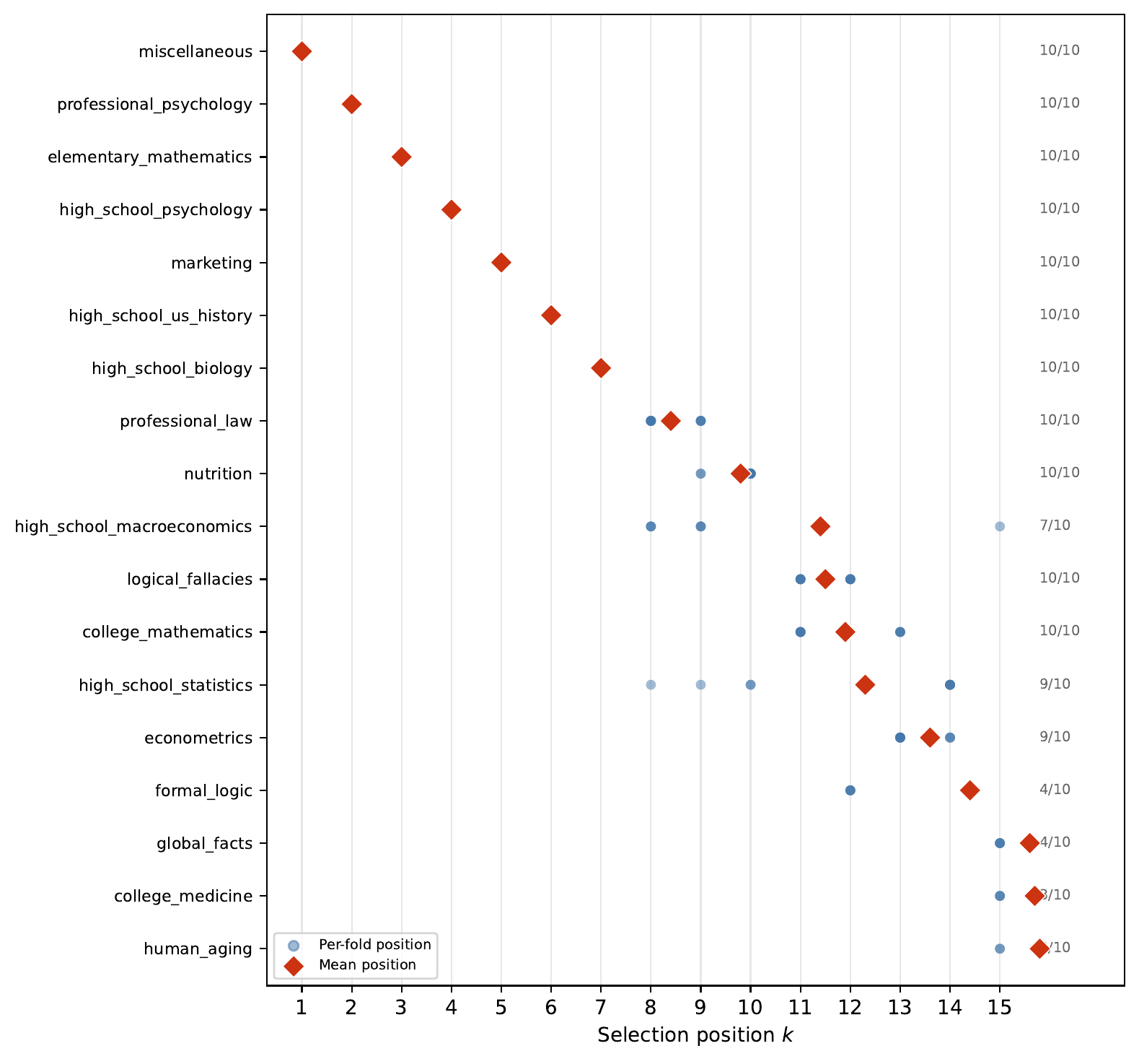
The hero image up top is what MI picks on MMLU, with selection positions averaged across the 10 folds (red diamonds) and per-fold positions in light blue. The first nine picks are identical across all 10 folds. The picks themselves are sensible: miscellaneous, professional_psychology, elementary_mathematics, high_school_psychology, marketing. A deliberately broad sweep of the MMLU domain.
We’re not alone
A few neighbors in this corner of the literature:
- tinyBenchmarks reduces redundancy within a benchmark by selecting representative examples.
- Sloth fits low-dimensional latent skills across benchmark families to predict performance.
- BenchBench diagnoses agreement among benchmarks via meta-benchmarking.
- BenchPress is the closest spiritual neighbor. It empirically observes that benchmark scores can be interpolated. Our entropy step turns out to be exactly pivoted Cholesky on \(\Sigma\), which is more or less what BenchPress does, but information-theoretically motivated rather than empirical.
One application: ranking a new benchmark
The same machinery applies in the dual. Instead of selecting benchmarks from a fixed pool, you can rank a new benchmark by its marginal MI gain against the incumbents. We tried this on the recently proposed ProactBench (arXiv:2605.09228), which decomposes conversational proactivity into Emergent, Critical, and Recovery axes. Recovery, assistance the user didn’t explicitly ask for, turns out to be weakly correlated with everything else (\(\bar r = 0.51\) vs. \(0.64\)–\(0.97\) for the standard benchmarks), and greedy entropy on the 9×9 correlation matrix ranks it #2 out of 9, ahead of every existing benchmark in the comparison. A clean example of when adding a new benchmark is actually worth the GPU time.
Paper: arXiv:2605.02209 · Workshop talk slides · Code and score matrices: github.com/smolix/benchmark-selection.