The code to our LDA implementation on Hadoop is released on Github under the Mozilla Public License. It’s seriously fast and scales very well to 1000 machines or more (don’t worry, it runs on a single machine, too). We believe that at present this is the fastest implementation you can find, in particular if you want to have a) 1000s of topics, b) a large dictionary, c) a large number of documents, and d) Gibbs sampling. It handles quite comfortably a billion documents. Shravan Narayanamurthy deserves all the credit for the code. The paper describing an earlier version of the system appeared in VLDB 2010.
Some background: Latent Dirichlet Allocation by Blei, Jordan and Ng, 2003 is a great tool for aggregating terms beyond what simple clustering can do. While the original paper showed exciting results it wasn’t terribly scalable. A significant improvement was the collapsed sampler of Griffiths and Steyvers, 2004. The key idea was that in an exponential families model with conjugate prior you can integrate out the natural parameter, thus providing a sampler that mixed much more rapidly. It uses the following update equation to sample the topic for a word.
\[p(t|d,w) \propto \frac{n^∗(t,d) + \alpha_t}{n^*(d) + \sum_{t'} α_{t'}} + \frac{n^∗(t,w) + \beta_w}{n^∗(t) + \sum_{w'} \beta_{w'}}\]
Here \(t\) denotes the topic, \(d\) the document, \(w\) the word, and \(n(t,d)\), \(n(d)\), \(n(t,w)\), \(n(t)\) denote the number of words which satisfy a particular (topic, document), (document), (topic, word), (topic) combination respectively. The starred quantities such as \(n^*(t,d)\) simply mean that we use the counts where the current word for which we need to resample the topic is omitted.
Unfortunately the above formula is quite slow when it comes to drawing from a large number of topics. Worst of all, it is nonzero throughout. A rather ingenious trick was proposed by Yao, Mimno, and McCallum, 2009. It uses the fact that the relevant terms in the sum are sparse and only the \(\alpha\) and \(\beta\)-dependent terms are dense (and obviously the number of words per document doesn’t change, hence we can drop that, too). Dropping the common denominator \(n^*(d) + \sum_{t'} α_{t'}\) we arrive at
\[p(t|d,w) \propto \frac{\alpha_t \beta_w}{n^∗(t) + \sum_{w'} \beta_{w'}} + n^∗(t,d) \frac{n^∗(t,w) + \beta_w}{n^∗(t) + \sum_{w'} \beta_{w'}} + n^*(t,w) \frac{\alpha_t}{n^∗(t) + \sum_{w'} \beta_{w'}}\]
Out of these three terms, only the first one is dense, all others are sparse. Hence, if we knew the sum over \(t\) for all three summands we could design a sampler which first samples which of the blocks is relevant and then which topic within each of these blocks. This is efficient since the first term doesn’t actually depend on \(n(t,w)\) or \(n(t,d)\) but rather only on \(n(t)\) which can be updated efficiently after each new topic assignment. In other words, we are able to update dense term in \(O(1)\) operations after each sampling step and the remaining terms are all sparse. This trick gives a 10-50 times speedup in the sampler over a dense representation.
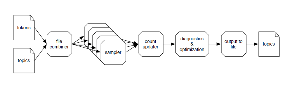
To combine several machines we have two alternatives: one is to perform one sampling pass over the data and then reconcile the samplers. This was proposed by Newman, Asuncion, Smyth, and Welling, 2009. While the approach proved to be feasible, it has a number of disadvantages. It only exercises the network while the CPU sits idle and vice versa. Secondly, a deferred update makes for slower mixing. Instead, one can simply have each sampler communicate with a distributed central storage continuously. In a nutshell, each node sends the differential to the global statekeeper and receives from it the latest global value. The key point is that this occurs asynchronously and moreover that we are able to decompose the state over several machines such that the available bandwidth grows with the number of machines involved. More on such distributed schemes in a later post.