class arrayHeap:
    # List of terms on array
    def __init__(self, probabilities):
        self.m = len(probabilities)            # sample size
        self.b = int(math.ceil(math.log(self.m,2))) # bits
        self.limit = 1 << self.b
        self.heap = numpy.zeros(self.limit << 1)    # allocate twice the size

        # allocate the leaves
        self.heap[self.limit:(self.limit + self.m)] = probabilities
        # iterate up the tree (this is O(m))
        for i in range(self.b-1,-1,-1):
            for j in range((1 << i), (1 << (i + 1))):
                self.heap[j] = self.heap[j << 1] + self.heap[(j << 1) + 1]

    # remove term from index (this costs O(log m) steps)
    def delete(self, index):
        i = index + self.limit
        w = self.heap[i]
        for j in range(self.b, -1, -1):
            self.heap[i] -= w
            i = i >> 1

    # add value w to index (this costs O(log m) steps)
    def add(self, index, w):
        i = index + self.limit
        for j in range(self.b, -1, -1):
            self.heap[i] += w
            i = i >> 1

    # sample from arrayHeap
    def sample(self):
        xi = self.heap[1] * numpy.random.rand()
        i = 1
        while (i < self.limit):
            i <<= 1
            if (xi >= self.heap[i]):
                xi -= self.heap[i]
                i += 1
        return (i - self.limit)

#Input: normalized probabilities, sample size
def sampleWithoutReplacement(p, n):
    heap = arrayHeap(p)
    samples = numpy.zeros(n, dtype=int) # result vector
    for j in range(n):
        samples[j] = heap.sample()
        heap.delete(samples[j])
    return samples

#Input: dense matrix p, resampling rate n
def sparsifyWithoutReplacement(p, n=1):
    (nr, nc) = p.shape
    res = scipy.sparse.lil_matrix(p.shape) # allocate sparse container
    for i in range(nr):
        tmp = sampleWithoutReplacement(p[i,:], n)
        weight = 1.0            # we start with full weight first
        for j in range(n):
            res[i,tmp[j]] = weight + (n-j - 1.0) * p[i,tmp[j]]
            weight -= p[i,tmp[j]]
    res *= (1/float(n))
    return res
Sometimes we want to compress vectors to reduce memory footprint or to minimize computational cost. For instance in deep learning we can accelerate operations by keeping only 2 out of 4 of all coefficients. This also occurs when we want to replace a probability vector by a sample from it. Without loss of generality, assume that our vector \(v\) has only nonnegative entries and that its entries sum up to 1, i.e. that it is a probability vector. If not, we simply apply our sampling scheme to the following:
\[v \leftarrow \|v\|_1^{-1} v\]
There are a few strategies one could use to obtain a sparse vector \(s\):
Sampling uniformly at random
For an n-dimensional vector simply use the sparsification rule: pick a random number \(j\) in \(\{1 \ldots n\}\). Set the j-th coordinate in the sparse vector to \(s_j \leftarrow n v_j\) and set all other terms \(s_{j'} = 0\). For k draws from this distribution, simply average the draws. This scheme is unbiased but it has very high variance since there’s a very high chance we’ll miss out on the relevant components of v. This is particularly bad if v only has a small number of nonzero terms, or if a small number of terms is large. Do not use this algorithm!
Sampling according to \(v\) at random
A much better method is to draw based on the size of the entries in \(v\). That is, treat \(v\) as a probability distribution and draw from it. If we draw coordinate \(j in \{1 \ldots n\}\) then set the j-th coordinate of the sparse vector to \(s_j = 1\) and all other terms to 0. As before, for k draws from this distribution, simply average. The advantage of this method is that now the entries of s are within the range [0, 1] and that moreover we hone in on the nonzero terms with high weight. But we can do better.
Sampling according to \(v\) with replacement
The key weakness in the above methods can be seen in the following example: for a vector of the form \(v = (0.99, 0.005, 0.005, 0, 0, \ldots , 0)\) we would need to perform many samples with replacement from v until we even draw a single instance from the second or third coordinate. This is very time consuming. However, once we’ve drawn coordinate 1 we can inspect the corresponding value in \(v\) at no extra cost and there’s no need to redraw it.
Enter sampling with replacement: draw from \(v\), remove the coordinate, renormalize the remainder to \(1\) and repeat. This gives us a sample drawn without replacement (see the code below which builds a heap and then adds/removes things from it while keeping stuff normalized). However, we need to weigh things differently based on how they’re drawn. Here’s what you do when drawing k terms without replacement:
\[\text{for $i=1$ to $k$ update } s_j \leftarrow \frac{k-i}{k} v_j + \frac{\gamma}{k} \text{ and } \gamma \leftarrow \gamma - v_j\]
Here we initialize \(\gamma=1\) and \(j\) is the index of the item drawn at the i-th step. Below is some (I hope relatively bug-free) sample code which implements such a sampler. As far as I recall, I found partial fragments of the heap class on stackoverflow but can’t quite recall where I found it and who to attribute this to. This could be made more efficient in C++ but I think it conveys the general idea.
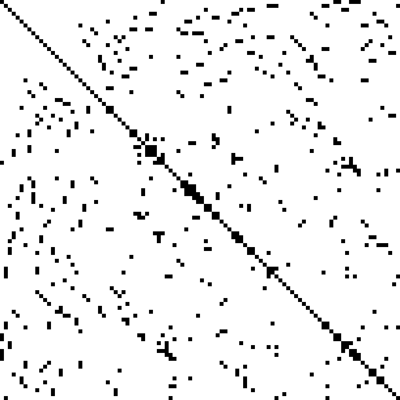
PS: The figure of a sparse matrix is from Wikipedia. .