Imagine you want to design some algorithm to detect cancer. You get data of healthy and sick people; you train your algorithm; it works fine, giving you high accuracy and you conclude that you’re ready for a successful career in medical diagnostics. Not so fast. Many things could go wrong. In particular, the distributions that you work with for training and those in the wild might differ considerably.
This happened to an unfortunate startup I had the opportunity to consult for many years ago. They were developing a blood test for prostate cancer, a disease that affects mainly older men. Luckily for them they’d managed to obtain a fair amount of blood samples from patients. It is considerably more difficult, though, to obtain blood samples from healthy men, mainly for ethical reasons. For instance, what do you do with positives? To compensate for that, they asked a large number of students on campus to donate blood and they performed their test. Then they asked me whether I could help them build a classifier to detect the disease. I told them that it would be very easy to distinguish between both datasets with probably near perfect accuracy. After all, the test subjects differed in age, hormone level, physical activity, diet, alcohol consumption, and many more factors unrelated to the disease. This was unlikely to be the case with real patients: Their sampling procedure had caused an extreme case of covariate shift that couldn’t be corrected by conventional means. In other words, training and test data were so different that nothing useful could be done and they had wasted significant amounts of money.
In general the situation is not quite so dire. Assume that we want to estimate some dependency \(p(y|x)\) for which we have labeled data \((x_i,y_i)\). Alas, the observations \(x_i\) are drawn from some distribution \(q(x)\) rather than the ‘proper’ distribution \(p(x)\). If we adopt a risk minimization approach, that is, if we want to solve
\[\mathop{\mathrm{minimize}}_f \frac{1}{m} \sum_{i=1}^m l(x_i,y_i,f(x_i)) \frac{λ}{2} \|f\|^2\]
we will need to re-weight each instance by the ratio of probabilities that it would have been drawn from the correct distribution. That is, we need to reweight things by \(\frac{p(x_i)}{q(x_i)}\). This is the ratio of how frequently the instances would have occurred in the correct set vs. how frequently it occurred with the sampling distribution \(q\). It is sometimes also referred to as the Radon-Nikodym derivative. Such a method is called importance sampling and the following derivation shows why it is valid:
\[\int f(x) dp(x) = \int f(x) \frac{dp(x)}{dq(x)} dq(x)\]
Alas, we do not know \(\frac{dp(x)}{dq(x)}\). Vefore we can do anything useful we need to estimate the ratio. Many methods are available, e.g. some rather fancy operator theoretic ones which try to recalibrate the expectation operator directly using a minimum-norm or a maximum entropy principle. However, there exists a much more pedestrian, yet quite effective approach that will give almost as good results: logistic regression.
After all, we know how to estimate probability ratios. This is achieved by learning a classifier to distinguish between data drawn from \(p\) and data drawn from \(q\). If it is impossible to distinguish between the two distributions then it means that the associated instances are equaly likely to come from either oneof the two distributions. On the other hand, any instances that can be well discriminated should be significantly over/underweighted accordingly. For simplicity’s sake assume that we have an equal number of instances from both distributions, denoted by \(x_i \sim p(x)\) and \(x_i' \sim q(x)\) respectively. Now denote by \(z_i\) labels which are \(1\) for data drawn from \(p\) and \(-1\) for data drawn from \(q\). Then the probability in a mixed dataset is given by
\[p(z=1|x)=\frac{p(x)}{p(x)+q(x)}\]
Hence, if we use a logistic regression approach which yields \(p(z=1|x)=\frac{1}{1+ e^{-f(x)}}\), it follows (after some simple algebra) that
\[\frac{p(z=+1|x)}{p(z=−1|x)} = e^{f(x)}.\]
Now we only need to solve the logistic regression problem (or use some convenient AutoML tool such as AutoGluon)
\[\mathop{\mathrm{minimize}}_f \frac{1}{2m} \sum_{(x,z)} \log\left[1+\exp(−zf(x))\right]+\frac{\lambda}{2} \|f\|^2\]
to obtain \(f\). Subsequently we can use \(e^{f(x_i)}\) as covariate shift correction weights in training our actual classifier. The good news is that we can use an off-the-shelf tool to deal with a decidedly nonstandard estimation problem. Note that the weights \(e^{f(x_i)}\) can be quite a bit off. This is fixable, e.g. by using an estimator that isn’t prone to this, or by using conformal methods. But that’s a topic for another day.
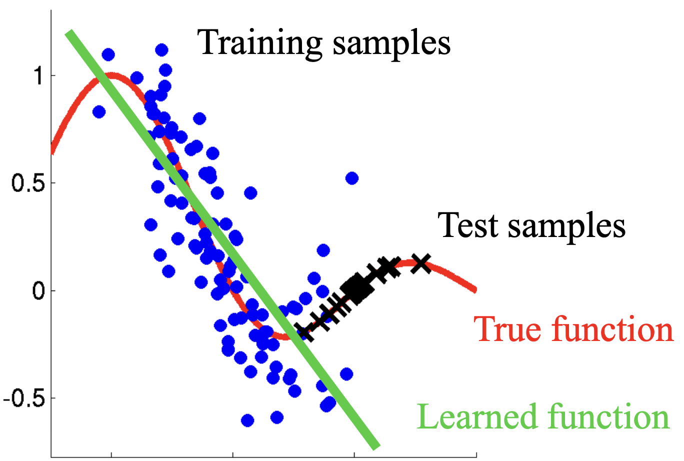
PS: The figure up top (which has been copied all over the internet, often without attribution) is likely due to Masashi Sugiyama.